
|
Instructions for Zefsa II |
>Decide where the main directory for
ZEFSA
II will be. A big, local disk would be the ideal location.
Make a directory called zefsaII. This directory will contain
all of the ZEFSA II code. Move the files zefsaII.tar.gz
and examples.tar.tz
into that directory. Then type
gunzip *.gz
tar -xvf *.tar
This will unzip and untar the ZEFSA
II files. Type
setenv ZEFSADIR directory
where directory is the
fully-qualified pathname of your zefsaII directory, with no
trailing slash.
You next need to compile the ZEFSA II
source codes to make executables. Go into the zefsaII/src directory.
Examine the file "Makefile" to ensure that it will work on your system.
You will need either a valid cc or gcc ANSI C compiler. Then type
make clean
make banneal
make temper
make compute_PXD
make check_PXD
make xtl_to_zef
make do_hist.ex
Now that the executables have successfully
been generated, move them to the bin directory
mv banneal ../bin
mv temper ../bin
mv compute_PXD ../bin
mv check_PXD ../bin
mv xtl_to_zef ../bin
mv do_hist.ex ../bin
If you require any other executables, compile
and move them to the bin directory as well.
Now, let's say that you are going to solve
the structure called new1. The first action you need to take is to
construct the input diffraction pattern for ZEFSA II. There
is a script to help you do this in the $ZEFSADIR/pxd directory. First
create a .xtl file (using Cerius2, for example) with the unit cell and
symmetry that you want. Place nT atoms at arbitrary or random locations
in this unit cell, where nT is the number of crystallographically distinct
T-atoms (e.g. Si) you want. Copy the file input.xtl that you just
made to the $ZEFSADIR/pxd directory. Now edit the file gen.input.
You need to change the -100 in the line
-100
# USER SUPPLIED actual n of atoms (density)
to the total number of T-atoms you want
in the unit cell (i.e. the T-atom density times the unit cell volume).
Next you need to change the -200 in the line
-200
# USER SUPPLIED random seed
to any positive integer. This is
the random number seed used by ZEFSA II. The first value of
the seed could be 1. It could then be incremented for each succeeding
runs. The xtl_to_input script by
default will create all refelctions
out to two theta = 50 degrees for a Cu Kalpha wavelength of 1.54056.
You will need to modify these values on lines 34 and 35 of the script should
you want different ones.
Peaks closer than 0.1 degrees are combined into composite peaks.
If the "comp" flag is given, the two theta
tolerance on whether to combine peaks is specified by the "sep" parameter
on line 35, and the tolerance can be specified on the d-spacings
by using the "dcomp" flag instead. Peaks in the
range from "min" to "max" are
output.
(For users of previous versions of
ZEFSA II:
the generic.pxd file is now automatically generated and
no longer required to be supplied by the user.)
Now in the $ZEFSADIR/pxd directory type
xtl_to_input new1 input
This will create the file new1.pxd.
You will get two lines of error messages about "ERROR: EOF". This
will happen three times. This is ok. Any other ERROR messages
are serious and must be fixed. If all is well, the files new1.pxd and
new1.1 will now exist.
The first line of new1.pxd is one of the
following
X-RAY lambda
NEUTRON lambda
BOTH X-ray_lambda neutron_lambda
Where lambda is the wavelength of the
radiation. The default new1.pxd is setup for X-RAY scattering
with a Cu Kalpha source. If you have, for example, synchrotron data,
change the wavelength to the appropriate value. The
second line of the file contains the number of reflections in the file.
Each line after that contains h,k,l, multiplicity, I_xray(h,k,l), I_neutron(h,k,l)
if it exists, and the weight of the peak.
In some rare cases, the file new1.pxd may have
a higher symmetry, i.e. larger values of the multiplicities,
than it should.
This rare condition can be avoided by using a zero merging
distance in the gen.input file before running xtl_to_input
and editing the generated file new1.1 to
use the correct merging distance.
The file new1.pxd lists all of the reflections and multiplicities. The intensities are random, however. You need to copy your experimental intensities for each hkl reflection into this file. If the intensity in new1.pxd for a given hkl is negative, this reflection has been grouped into a composite peak. Composites occur because the spacing between distinct peaks is too small to resolve experimentally. So, all peaks close to each other are grouped into a single composite peak. All of the reflections that have been grouped into a composite have a negative -1 intensity except for the last one. So, sum up the experimental intensities of all the relfections in the composite and place this summed intensitiy in the last reflection of the group. Remember, the intensities in this file must be multiplied by the multiplicities.
The last column of the file new1.pxd is
the weight of the peak. Larger weights mean the peak intensity is
more uncertain and should be counted less in the comparision between experiment
and calculation. Typically, weights of 1 are used for intensities
below 100. A weight of 2 is used for 100 < I(hkl) < 200.
A weight of 3 is used for 200 < I(hkl) < 300. A weight of 4
is used for 300 < I(hkl) < 500. A weight of 5 is used for 500
< I(hkl) < 1000. Remember that the maximum I(hkl) should be
scaled to 1000.
There are some parameters that you can vary in the pxd creation script xtl_to_input. The default values are quite reasonable. These parameters are given as command line arguments to the program compute_PXD within the script. The parameter "sep" is the maximum separation between peaks that will be grouped into composites. It should be approximately the full width at half maximum experimental resoluion (in degrees). Any relfections with intensity below "int" will not be included. This should always be 0.0 (especially since this script does not know the structure and hence does not know the true intensities). Only reflections with two theta between "min" and "max" will be output.
It is very important that the file new1.pxd be valid. It is worthwhile to recheck the validity of this file.
This script xtl_to_input has also made
the other required input file for ZEFSA II. This file is called
"new1.1". Examine it to make sure it is ok. If you have no
template molecules, create a final line of this file that contains the
word "END". If templates, place the number of templates and the molecular
information at the end of the file, followed by an "END". For two
templates, one would use
n_mol
MOLECULE phi_max phi_min n_atoms
# for molecule 1
atom_type 1
x y z Debye_Waller occupancy
atom_type 2
x y z Debye_Waller occupancy
.
.
.
atom_type n_atom x y z
Debye_Waller occupancy
MOLECULE phi_max phi_min n_atoms
# for molecule 2
atom_type 1
x y z Debye_Waller occupancy
atom_type 2
x y z Debye_Waller occupancy
.
.
.
atom_type n_atom x y z
Debye_Waller occupancy
END
n_mol is the number of molecules.
phi_max and phi_min are the maximum and minimum angular displacements (in
degrees) of each molecule. n_atoms is the number of atoms in the molecule.
The information about the atoms in molecule is listed as above. An
example atom line would be
C -0.005282 3.653390 1.076101
1.0000 0.2500
The coordinates of the atoms in the molecule
are given in real space, in Angstroms. The molecule will be rigidly
rotated and translated by ZEFSA II. Symmetry will be applied
to the molecule to generate all of the symmetrically equivalent templates.
So, if the molecular density were known to imply only one molecule per
unit cell on average, the occupancy should be set at 1/(number of elements
in the space group). The example line above was for the space P2/m,
which has four elements. A Debye Waller factor of 1.0 is a good default
value.
Example .pxd and .1 files can be found in the examples directory. The files new.pxd and new.1 could be created by copying and modify an example rather than running the scripts described above. The script xtl_to_input needs to be run only once for a new structure. Input files for multiple runs (changing the random number seed, density, etc) can be created by simply copying the new1.1 file to new1.2 and making the one or two required changes on new1.2.
If you are unsure about the exact density,
space group, or number of unique T-atoms, make multiple input files.
One for each possible combination of density, space group, nT, etc.
Always try simulated annealing first when solving a structure. This is because simulated annealing is somewhat easier to set up. If it is successful, it is also faster. Typically, several simulated annealing runs would be done on a given input file, changing only the random number seed. If the structure is not solved in, say, 10 runs, then parallel tempering should be attempted.
To run the simulated annealing, you first need to set up a data directory. Create a directory such as $ZEFSADIR/new1. Then in that directory, create the directories run1. Copy new1.1 and new1.pxd to ZEFSADIR/new1/run1. Now create nine copies of new1.1. Call them new1.2, new1.3, ..., new1.10. Now edit the files $ZEFSADIR/new1/run1/new1.* to make the random number seeds different. Perhaps use seed=1 for new1.1 , seed = 2 for new1.2, and so on.
You can now do the runs! You can set up a batch file to do all the runs. The following would work:
#!/bin/sh
for x in 1
do
cd run$x
for y in 1 2 3 4 5 6 7 8 9 10
do
nice -19 ../../bin/banneal < new1.$y
mv messages messages.$y
mv hist.oogl hist.oogl.$y
done
cd ..
done
This file could be called "go". It
should be in the $ZEFSADIR/new1 directory. The file must be made
executable by typing
chmod +x go
Then you can run the script with
./go >/dev/null &
After some time, you will have ten output
files. The files messages.* will list the coordinates and energies
produced by the simulated annealing. You can view the output graphicaly.
To see the output of new1.1, type
geomview
hist.oogl.1
Geomview must be installed for this to
work. Also, the file dodec3.off must be in the same directory as
the hist.oogl.1 file in order for geomview to work properly (copy it from the
$ZEFSADIR/share directory). Note
that the geomview command can be executed even if the run is not yet
complete; the data is written continuously to the file hist.oogl and can
be viewed at any time. The molecular templates will be displayed
in this output if they are present. The templates created by
symmetry are present, but are not displayed.
If you are doing many runs, you may
find it difficult to deal with the large amount of output data. There
are some old programs in the file $ZEFDIR/scan to help with this.
These programs will collect the topologically unique structures produced
by very many runs. These programs can be compiled with
make clean
make scan3d
make scan3d_connected
make display3d
Two variables need to be set in the file
scan_it to begin the scanning. First, change the value of nT from
5 to your value in the line
n=5 # USER SUPPLIED
Next change the run directory from new1
in the line
rundir="new1"
# USER SUPPLIED
Copy the file start_n5.dat to run directory
$ZEFSADIR/$rundir. Change the "5" in the name of the file to your
value of nT. Three things need to be changed in this old-format file.
First, change the values of nT, number of symmetry operators, and number
of total T-atoms in the line
5
4 12
Change the next line to have the number
"4" nT times. Finally, change the a,b,c; alpha, beta, gamma; and
space group operators to those for your system. This information
can be copied from the file new1.1. Finally, create nT lines containing
the number "1" following the space group operators.
Now type scan_it in the directory $ZEFSADIR/scan.
This will collect all of the run data into one big file fort.2.
If you are running with non-standard parameters, you may need to change
the number 39 to something else in the file scan_it in the line
tail -n +39 .... This line
is deleting the first 38 lines in the run data files.
If that is too few or
too many lines for a run with non-standard parameters,
scan_it may produce mangled output.
Now
type scan3d.ex. Input the maximum energy for which you would like
to see structures (structures with energies greater than this will not
be collected). You may wish to redirect the output to a file, such
as
scan3d.ex > run1.scanout
Copy the file fort.3 to run1.scan.
If you want to include only three-dimensionally connected structures,
type scan3d_connected.ex instead.
Finally, to create postscript versions of the collected output, use display3d.ex.
First, copy fort.3 to fort.2, then type display3d.ex
Give a title for the output. Then type 1. Then type the same
maximum energy input to scan3d.ex.
After this, you should have the following
files
run1.scanout
run1.scan
pos*.ps
You can view the structures and the coordination sequences by printing the PostScript files pos*.ps. You can also view the structures on the screen with any PostScript viewer. To figure out which run produced a given pos*.ps unique structure, you can search through the runs to find the energy "e saved". Omit the last digit, which may be rounded.
For some reason, display3d sometimes does
not make all the bonds it should. Also, note that the bonds created
by scan3d and display3d are with an old algorithm. Only for very
good structures is the old algorithm be equivalent to that in ZEFSA
II.

The output can be collated with the scan_it
script described above. Simply create a directory $ZEFSADIR/examples/LTL/run1.
Copy the message file to run1/message.1. Then from the $ZEFSADIR/scan
directory, run the scan_it script. You will need to set the rundir
variable in that script as well as
the value of nT. Note that the file start_n2.dat
already already exists in the directory $ZEFSADIR/examples/LTL. Then
type
scan3d.ex
Enter 1000 as the maximum energy value.
Several topologically unique structures may be collected from the
run. The lowest one, found at the lowest temperature, should be LTL.
The coordination sequence for LTL is
4 9 17 29 46
69 98 131 162 187 752
4 10 21 35 49
66 89 117 150 190 731
1483
Another good example is SSZ35. This
is a material made by Stacey I. Zones at Chevron. This material is
somewhat harder to solve than LTL because it contains 8 unique T-atoms
in the low-symmetry setting derived by the inital indexing of the
diffraction pattern. The diffraction data in $ZEFSADIR/examples/SSZ35 is
real synchrotron data. Again, edit the file ssz.1 to set the correct
value of the data files directory. Then run simulated annealing:
$ZEFSADIR/bin/banneal
<ssz.1
After half an hour
or so, the hist.oogl and message files will be created. You
can view the output graphically with the command
geomview
hist.oogl.
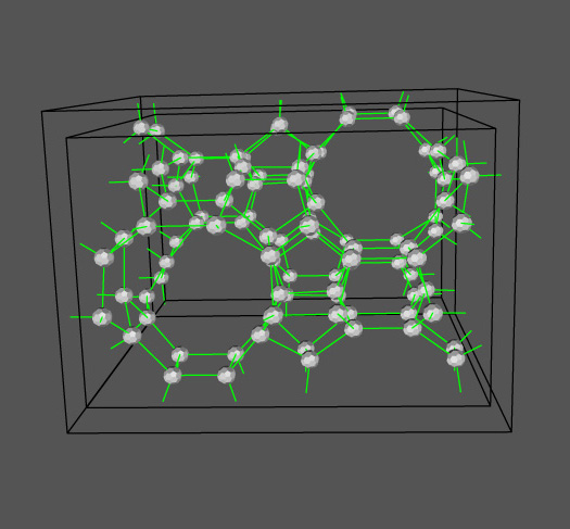
At the very end the SSZ35 structure should
appear. (Again, multiple runs of ZEFSA II may be needed
on unlucky computers.) You may see that some T-atoms have 4 green
bonds in addition to a blue bond. The green bonds are real "bonds"
created by ZEFSA II. The blue bonds are repulsive interactions
between T-atoms that are a little too close. Further refinement of
the structure (e.g. by DLS76 or more runs with ZEFSA II) would tend
to remove these repulsive interactions.

The results can be collated with $ZEFSADIR/scan/scan_it
as described above. Create the directory $ZEFSADIR/examples/SSZ35/run1.
Copy the message file to run1/message.1. Then from the $ZEFSADIR/scan
directory, run the scan_it script. You will need to set the rundir
variable in that script as well as the value of nT. Note that the
file start_n8.dat already already exists in the directory $ZEFSADIR/examples/SSZ35.
Then type
scan3d.ex
Enter 1000 as the maximum energy value.
Probably only one topologically unique structure will be collected from the
run. That structure should be SSZ35.
The coordination sequence for SSZ35 is
4 11 19 36 54
84 110 146 179 226 869
4 11 20 31 58
84 117 137 174 229 865
4 11 22 39 55
82 111 149 188 223 884
4 11 22 39 55
82 111 149 188 223 884
4 11 23 36 59
80 113 147 183 227 883
4 11 23 36 59
80 113 147 183 227 883
4 12 20 34 56
88 114 143 173 224 868
4 12 20 34 56
88 114 143 173 224 868
7004
A final example with a molecular template is MCM47.

The coordination sequence indicates that there are only four topologically
unique T-atoms, and the NMR data confirms this. Indeed, a higher
symmetry setting of Cmcm could have been used. Note that the real
material is layered, so that the long 3.9 A bonds are not present.
Interestingly, the template was not well localized by ZEFSA II.
For about 10% of the known zeolites, simulated annealing is unable to solve the structure. This is because the structure determination becomes more difficult with a greater number of unique T-atoms and an increased degree of merging. Simulated annealing should always be tried first on a new, unknown structure since it is somewhat easier to set up.
Parallel tempering is able to solve all of the known zeolite materials. In parallel tempering, serveral systems are simulated at different, constant temperates, and configurations are ocasionally swapped between systems at adjacent temperatures. This is in constrast to simulated annealing, where a single system is simulated at a temperature that is slowly decreased. Parallel tempering is an exact statistical mechanics method, whereas simulated annealing is an approximate method.
You will need three input files to run
parallel tempering. Two of them are the same as for simulated annealing.
First, create a directory $ZEFSADIR/new1/temper. Copy the new1.1
file created for simulated annealing to $ZEFSADIR/new1/temper/new1.temper.
Copy the file new1.pxd to $ZEFSADIR/new1/temper/new1.pxd. The temperatures
and acceptance ratio information in new1.temper are ignored in parallel
tempering. Specifically, these lines from gen.input must be present but
are ignored
3.00 1.0 1.00 # max and min proposed
move amplitude (Angstroms)
# and adjust factor
300.0 5.0 1
# initial temp / min temp / Sweeps in init heating
0.2 0.3
# acceptance ratio that defines melted phase
0.80
# alpha: temperature reduction factor
The line
5 2 100
# Therm Sweeps / SA steps / granularity
in new1.temper that contains the termalization
length, number of
steps, and granularity is used.
Typically, no termalization steps are
needed. A total of approximately
steps * granularity Monte Carlo moves will be
performed on each system. A good
choice for the new value of this line is
0 1000 1
# Therm Sweeps / MC steps / granularity
A separate file named "temperatures" must
also be created in
$ZEFSADIR/new1/temper. The format
of this file is
n
T_1 radius_1 update_probability_1 [d_phi_1]
.
.
.
.
T_n radius_n update_probability_n [d_phi_n]
p_update-vs-swap
The first line of this file contains the number of systems in the parallel tempering scheme. Typically, this should be 5 or 6. The next lines list the temperature, proposed move amplitudes, and relative probability of updating the system. If molecular templates are included the in system, the proposed rotation amplitude (in degrees) is listed in the last column. The last line of the file contains the probability of updating a system instead of performing a swapping event. A good choice is 0.9. T_1 is the lowest temperature, and T_n is the highest temperature. The lowest temperature should be the lowest one used in the simulated annealing runs. The highest temperature should be the highest one used in the simulated annealing runs. The intermediate temperatures should be such that the energy histograms of system i and system i+1 overlap. This criterion is what actually specifies the number of systems once the maximum and minimum temperatures have been chosen. Choosing 5 or 6 systems and spacing the temperatures exponentially between the minimum and maximum usually works well.
Parallel tempering can be run with the
command
$ZEFSADIR/bin/temper
< new1.temper
After some time, several files will be
created. The message file contains the output associated with system
0 (the lowest temperature system). Also created will be the files
hist_*.oogl. These are the .oogl files for the systems at the different
temperatures. Most useful will be the file hist_0.oogl. Finally,
the files hist_*.ene are also created. These files contain the energy
and framework position information for each of the systems.
You can view the output graphically with
the command
geomview
hist_0.oogl
The molecular templates will be displayed
in this output if they are present. The templates created by
symmetry are present, but are not displayed.
Alternatively, the .oolg file
can be created and viewed from the associated .ene file with the command
oolg_confs:
cat
new1.oogl hist_0.ene | $ZEFSADIR/oogl_confs | geomview -c -
The file new1.oogl is a copy of new1.temper
except that the last lines giving the silicon positions have beem removed.
The final line containing the "END" has been removed as well.
The .oogl file displayed this way will not contain any molecular templates.
The histograms of the energies of each system in parallel
tempering can be constructed
with the do_hist script. The do_hist script is in the
directory $ZEFSADIR/src. The values of the
variables max, min, and dx may need to be modified
to suit the structure being solved.
The variables min and max define the minimum and maximum
energy values of the histogram. The variable dx defines the width of the
histogram bins. A smaller dx gives a finer detail.
A larger dx gives a smoother looking histogram. These values show up in the
lines
set min=-700 # USER SUPPLIED
set max=2000 # USER SUPPLIED
set dx=10 # USER SUPPLIED
in the file $ZEFSADIR/src/do_hist. Finally, the do_hist script needs to
be modified if the number of systems is not n=6. The following line
foreach x (0 1 2 3 4 5) # 6 systems
should contain the numbers 0, 1, ..., n-1. To construct the histograms,
simply type
$ZEFSADIR/src/do_hist
This will create the files hist_*.dat. These files can be plotted with
a program, as in
xmgr hist_*.dat
An example parallel tempering run can be found in $ZEFSADIR/examples/MFI/temper. MFI is the most complex zeolite known, and its structure could not be found easily with simulated annealing. We decided to use 6 systems, with the temperatures spaced between 8 and 160. We updated the systems at the two lowest temperatures twice as often as those at the highest temperatures, since the correlation times at the lower temperatures are longer. We choose the move amplitudes between 0.6 Angstroms at the lowest temperature and 2.0 Angstroms at the highest temperature. We choose a probability of performing a normal Monte Carlo move versus swapping of 0.9.
To run this example, first edit the line
/usr/scratch2/mwdeem/zefsaII/DIST/share
# data path
in $ZEFSADIR/examples/MFI/temper to reflect
where the data files are. Then parallel tempering can be run from
ZEFSADIR/examples/MFI/temper with the command
$ZEFSADIR/bin/temper < mfi.temper
After an hour or so, the .oogl, .ene,
and messages files should be created. They can be viewed as desribed
above:
geomview hist_0.oogl
The results can be collated with
$ZEFSADIR/scan/scan_it as described above. Create the directory $ZEFSADIR/examples/MFI/temper/run1. Copy the message file to
run1/message.1. Then from the $ZEFSADIR/scan directory, run the scan_it script. You will need to set the rundir variable in that script
as well as the value of nT. Note that the file start_n12.dat already already exists in the directory $ZEFSADIR/examples/MFI/temper.
Then type
scan3d.ex
Enter 1000 as the maximum energy value. Probably
only one topologically unique structure will be collected from the run. That structure should be MFI. The coordination sequence for MFI
is
4 11 22 36 61 93 120 154 200 255 956
4 11 23 39 62 93 119 153 204 254 962
4 12 21 36
61 90 122 159 196 251 952
4 12 21 37 63 90 121 155 201
253 957
4 12 22 38 59 92 125 159 202 250 963
4 12 22 39 64 91 117 158 209 247 963
4
12 22 40 61 88 124 156 197 253 957
4 12 22 41 61
88 125 159 198 250 960
4 12 23 37 62 91 120 157 206 250
962
4 12 23 38 59 89 126 161 196 246 954
4 12 24 38 56 90 132 164 193 241 954
4 12 24 38
63 93 123 157 206 247 967
11507
The histogram from this parallel tempering run can be created with the command
$ZEFSADIR/src/do_hist
The histograms can be plotted with the command
xmgr hist_*.dat
For the MFI example, the temperatures were not well-optimized. In
particular, the histograms of systems 2 and 3 do not overlap very much. The structure was still relatively easy to solve, however, even with these
non-optimal temperatures.
